
Forest Edge Management as a Bioenergy Resource – Documentation of Analysis
Author: Erlend Torheim Bjelkarøy, Fredrikstad Municipality
The analysis of the potential for bioenergy from forest edge management was conducted using the tools Safe FME for data processing and ESRI ArcGIS for presenting data in an online map. This note documents the procedure of the analysis. The steps described are not software-dependent and can thus be developed with most GIS tools. The base data in the analysis is a mix of open data and data available to «Norge Digitalt» partners. Partners who are not part of Norge Digitalt collaboration can purchase data commercially.
Read our best practices for replication:
In short, the analysis involves defining areas where forest edge clearing can be performed (e.g., along roads) and clipping these areas against NIBIO’s forest resource dataset in 16x16m grids (the SR16 dataset). Protected areas are excluded from the analysis results. Finally, the analysis results are presented at three levels:
- Aggregate per municipality
- Aggregate in 1km x 1km grids
- Detailed level (no aggregation)
In the analysis, we used forest clearing along roads, power lines, and crop edges for cultivated land. Datasets and distances are described in more detail later in this document.
Although the analysis is essentially a simple overlay analysis, a considerable amount of data processing has been done. In the TREASoURcE project, the FME project for data processing looks like this:
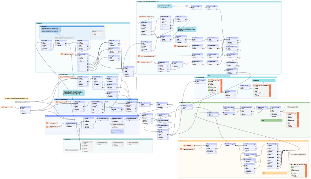
Figure 1: Model-based data processing in the FME Form software.
Each of the small blue boxes in Figure 1 represents a data processing step. It is difficult to provide a complete textual description of all the steps in the analysis. Those interested can receive the FME project by contacting Erlend Bjelkarøy at erlbje@fredrikstad.kommune.no.
In the documentation below, we will describe the analysis in general terms, step-by-step. We will also describe some of the parameters we used and the considerations we made along the way.
1. The Analysis: Step-by-Step
Below you will find a step-by-step description of the analysis, including the base data used, the properties of the base data, and how we have processed it.
1.1 Finding Areas for Side Clearing
Areas along cultivated land
For areas along cultivated land, we used the FKB AR5 dataset and land types 21, 22, and 23 (respectively fully cultivated land, surface cultivated land, and pasture). We used a 5-meter buffer outside all field edges.
Power line corridors
Data for power lines was downloaded from NVE (Norwegian Water Resources and Energy Directorate). In the attribute “nveNettnivaa,” there is a classification where level 1 is the transmission network (110 – 525kV), level 2 is the regional network (32 – 170kV), and level 3 is the distribution network (under 24kV). We used a buffer of 20 meters on each side for transmission network power lines, 15 meters on each side for regional network power lines, and 10 meters on each side for distribution network power lines. These buffer distances corresponds very well with what is visible as established power line corridors in aerial photos.
Along roads
As a basis for road data, we used FKB road (area/surface). By using the road surface instead of the centerline of the road, buffer areas can be created adjacent to the roadway. In the Norwegian Public Roads Administration’s handbook 610 “Standard for Road Maintenance” the following table is shown:
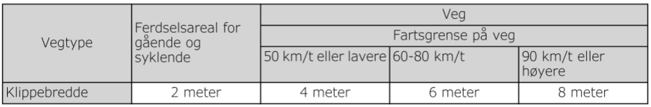
Figure 2: Table 12.2.2-2 – “Requirements for clearing width” from the Norwegian Public Roads Administration’s handbook “Standard for Road Maintenance”. «Klippebredde» means clearing distance.
The table is based on the speed limit on the road to indicate the cutting width. The road surface dataset does not contain speed limit information, and although it is possible to assign this information to the surfaces, we have for simplicity used the attribute “road category” which describes the ownership of the road:
P = private road
S = forest road
K = municipal road
F = county road
R = national road
E = European road
In the analysis, we assumed that roads with road category = P, S, and K have a cutting width of 4 meters, roads with road category = F and R have a cutting width of 6 meters, and roads with road category = E have a cutting width of 8 meters.
We have also explored the possibility of using the FKB Tractor Road Path dataset in the analysis but have not yet implemented this due to uncertainty in data accuracy in some areas.
1.2 Areas Excluded from the Analysis
Some areas are not suitable for logging due to conflicting interests such as protection and private property rights. Below we describe areas that are excluded from the areas suitable for forest clearing.
Riparian zones
Along streams, rivers, and lakes, it is desirable to preserve the riparian vegetation, both for the sake of the riparian zone’s function as a habitat, for erosion control, and the riparian vegetation’s ability to capture runoff.
As a basis for data, we used FKB water boundary/line objects, and lakes in FKB AR5 (land type 81). The table below shows criteria for data selection and corresponding buffer distances:
| Dataset | Selection based on attribute | Buffer distance |
FKB vann (water) | Objekttype = ElvBekk AND vannbredde = 1 eller 2 | 10m |
| Objekttype = ElvBekk AND vannbredde = 3 | 20m | |
| Objekttype = Elvkant OR Innsjøkant | ||
| AR5 | Arealtype = 81 |
Table 1: Criteria for data selection and corresponding buffer distances
The buffer distances above are based on a guide prepared by NVE and the County Governor in Hedmark and Oppland: brosjyre-om-skjotsel-av-kantvegetasjon-langs-vassdrag.pdf.
Nature conservation
Nature conservation areas, nature types mapped according to Handbook 13, and nature types mapped according to the NiN method are not suitable areas for logging. Here we used the conservation areas as they are in the datasets, with the exception of hollow oaks (NiN mapping, nature type code C01) which are reduced in circular diameter from 30m to 10m by setting a buffer of minus 10 meters.
We have requested data for Environmental Areas in Forests(«Miljøområder i skog») from the Norwegian Agriculture Agency without receiving a response. These data would also have been relevant conservation areas if we had access to them.
Gardens and parks
In residential/urban areas, the analysis excluded clearing along roads as these areas often involve gardens and parks associated with developed urban areas. To clip these areas, we used land type 11 (buildings) in the FKB AR5 dataset. These building areas were buffered 15 meters before being used as clipping areas.
1.3 Overlay of Areas for Side Clearing and SR16
By clipping away areas excluded from the analysis (chapter 1.2) from the areas for side clearing (chapter 1.1), we are left with the final areas we want to explore to find the potential for forest clearing. This is done by using the final areas as clipping polygons on the forest resource dataset SR16. SR16 can be downloaded from Geonorge.no, but this dataset is initially clipped so that it only covers contiguous forest areas. This creates gaps in the dataset, e.g., along field edges. Therefore, in consultation with experts at NIBIO (Norwegian Institute for Bio Economics), we obtained access to an SR16 dataset that is not clipped but is comprehensive for almost all land areas.
Due to data size considerations, we used raster data in the file exchange. The file we received contained only one “band,” meaning the dataset contained only one attribute at a time. Therefore, we had to combine two raster files, each containing the attribute “SRVOLMB” and “SRTRESLAG,” respectively biomass volume with bark per hectare, and tree species divided into spruce, pine, and deciduous forest.
For raster data to be clipped into smaller sizes than the pixel size of 16m x 16m, the raster data was converted to polygons with the attributes SRVOLMB and SRTRESLAG. Each grid was then calculated with new values to compensate for the clipping. The following formula was used:
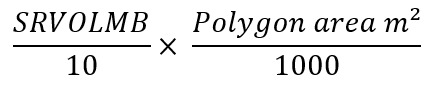
By dividing SRVOLMB by 10, we convert the biomass volume per hectare to biomass per decare(more common unit in Norway). The same calculation can be done by simplifying the formula as follows:

In addition, we added a calculation for each polygon that converts the biomass volume to energy value in MWt depending on the type of tree species. We used the following conversion factors:
- 1 m³ spruce = 1,65 MWh
- 1 m³ pine = 1,9 MWh
- 1 m³ deciduous trees = 2,1 MWh
2. Presentation of Data
The result of the analysis in an area the size of Østfold creates almost 2 million small polygons that are 16m x 16m or smaller. For such data to be presented in maps for large areas, we need to aggregate the data. We have done this at three levels:
- Level 1: no aggregation,
- Level 2: aggregate at 1km x 1km
- Level 3: aggregate at the municipal level
By controlling which layer is visible at different scales, we can present the data in a readable way at all scales.
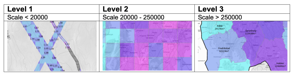
Table 2: Aggregation levels in relation to scale and map details
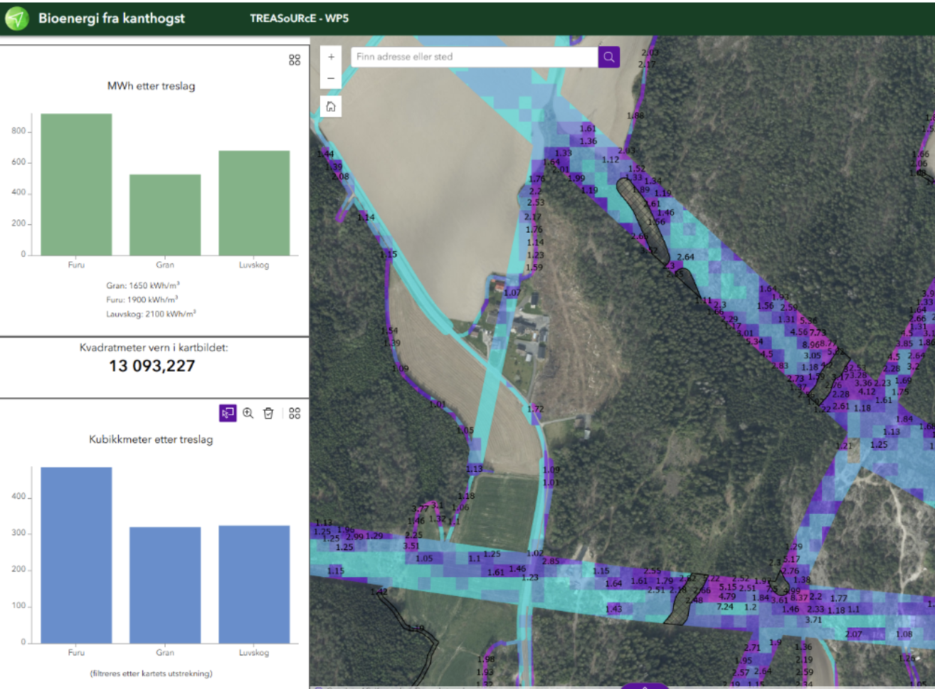
At level 1, we also chose to show areas excluded from the analysis (ref. chapter 1.2). These areas are shown as black hatches. The map is symbolized using values for the number of cubic meters of biomass within each area. Choropleth from light blue to purple/pink shows increasing numbers of cubic meters.
In addition, the map is presented as a dashboard showing graphs with information on the number of cubic meters and MWh. These graphs change depending on what is shown in the map view so that when you move around the map, the graphs update with information for the area shown.
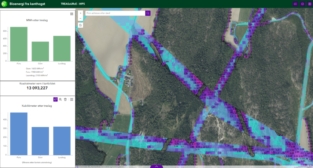
Figure 3: Screenshot of the map solution/dashboard that can be viewed online
When you zoom far into the map (scale level 1/no aggregation), it is also possible to filter by tree type by clicking on one of the bars in the graph showing cubic meters by tree species.
The map/dashboard can be viewed on the following website: https://arcgis.fredrikstad.kommune.no/portal/apps/experiencebuilder/experience/?id=3bb166572cc9485c824d88c1c8ceed81